Simulating GWAS data, a walkthrough

Load the library

library(simGWAS)

simGWAS needs some reference haplotype frequencies from control subjcets. These can be found by taking phased haplotypes from public data sources, or by phasing genotype data you may already have, for example using snphap.

For the purpose of this vignette, we will simulate some reference haplotypes. The final format is a data.frame with n columns of 0s and 1s indicating alleles at each of n SNPs, and collections of alleles in a row being a haplotype. A final column, named “Probability”, contains the fractional frequency of each haplotype. Note that haplotypes need not be unique, you can have one row per haplotype in a sample, and Probability set to 1/[number of haplotypes] = 1/(2*[number of samples]). The object we are creating will be called freq.

set.seed(42)
nsnps <- 100
nhaps <- 1000
lag <- 5 # genotypes are correlated between neighbouring variants
maf <- runif(nsnps+lag,0.05,0.5) # common SNPs
laghaps <- do.call("cbind", lapply(maf, function(f) rbinom(nhaps,1,f)))
haps <- laghaps[,1:nsnps]
for(j in 1:lag) 
    haps <- haps + laghaps[,(1:nsnps)+j]
haps <- round(haps/matrix(apply(haps,2,max),nhaps,nsnps,byrow=TRUE))

snps <- colnames(haps) <- paste0("s",1:nsnps)
freq <- as.data.frame(haps+1)
freq$Probability <- 1/nrow(freq)
sum(freq$Probability)

## [1] 1

Next, we need to specify the causal variants, and their effects on disease, as odds ratios. We create a vector CV with snp names that are a subset of column names in freq and a vector of odds ratios. In our simulated data, we pick two causal variants at random, with odds ratios of 1.4 and 1.2.

CV=sample(snps[which(colMeans(haps)>0.1)],2)
g1 <- c(1.4,1.2)

Now we simulate the results of a GWAS. There are two key functions, makeGenoProbList calculates genotype probabilities at each SNP conditional on genotypes at the causal variants, then est_statistic generates the vector of Z scores across all SNPs, conditional on the causal variants and their odds ratios.

FP <- make_GenoProbList(snps=snps,W=CV,freq=freq)
zexp <- expected_z_score(N0=10000, # number of controls
              N1=10000, # number of cases
              snps=snps, # column names in freq of SNPs for which Z scores should be generated
              W=CV, # causal variants, subset of snps
              gamma.W=log(g1), # odds ratios
              freq=freq, # reference haplotypes
              GenoProbList=FP) # FP above

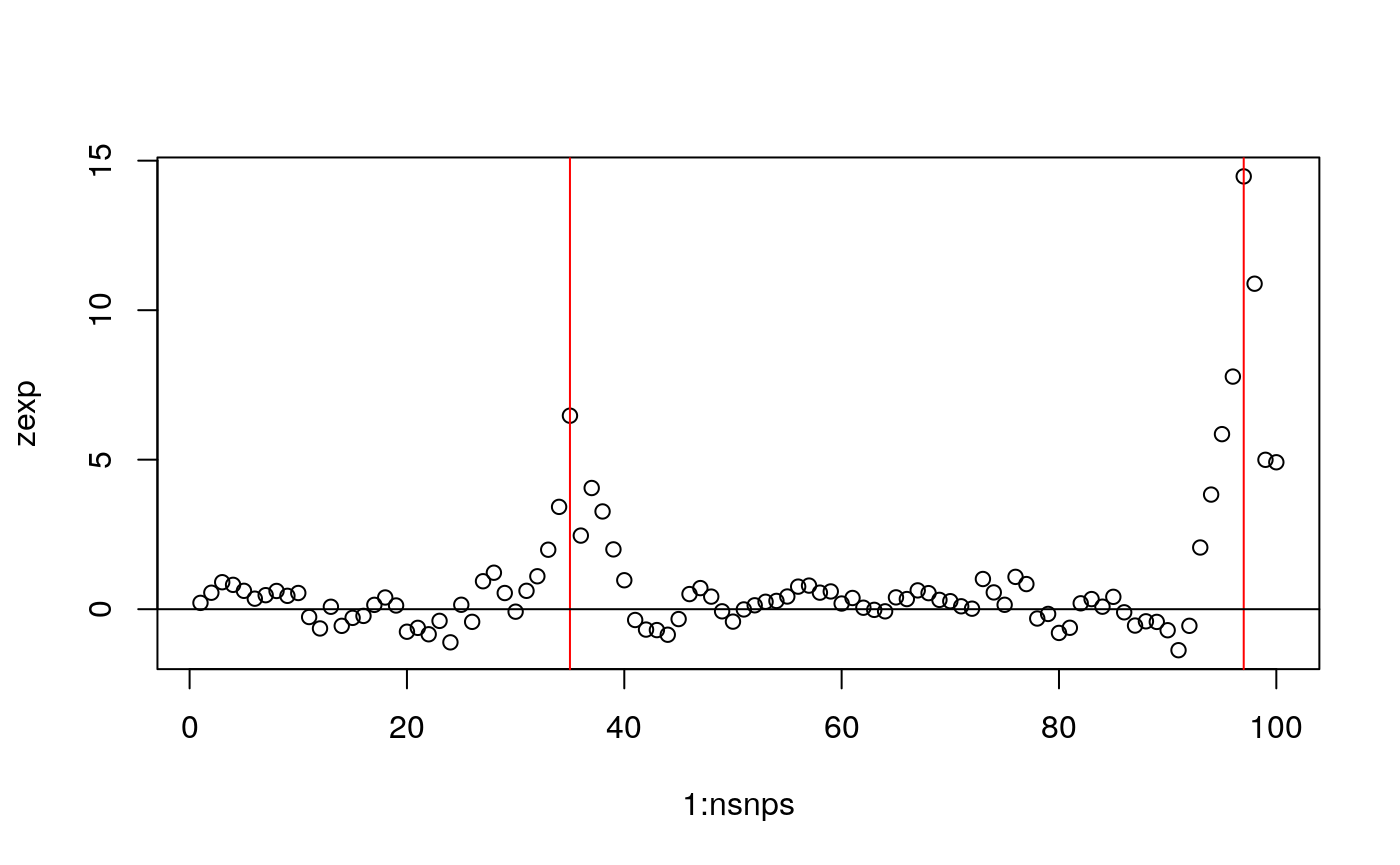
Ignoring spacing, this would produce results like, with red lines indicating where the causal variants are.

plot(1:nsnps,zexp); abline(v=which(snps %in% CV),col="red"); abline(h=0)

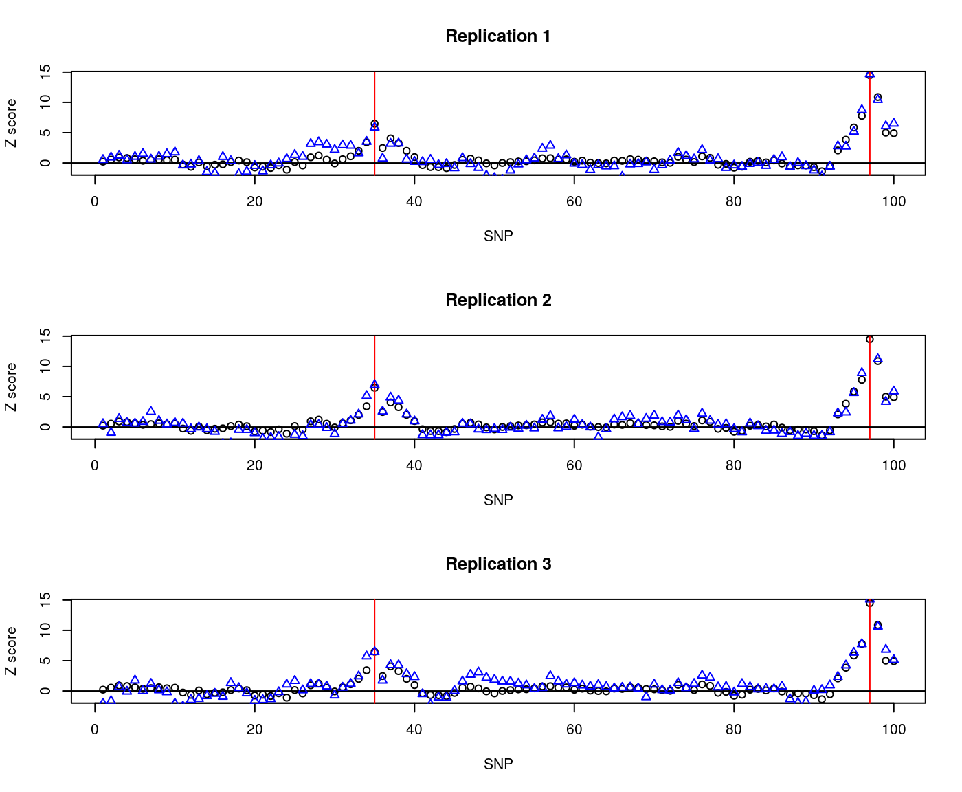
True GWAS statistics will vary about this expected value, and may be simulated by (one row per realisation)

zsim <- simulated_z_score(N0=10000, # number of controls
              N1=10000, # number of cases
              snps=snps, # column names in freq of SNPs for which Z scores should be generated
              W=CV, # causal variants, subset of snps
              gamma.W=log(g1), # log odds ratios
              freq=freq, # reference haplotypes
          nrep=3)

To see how these vary about the expected, we can overplot the two:

par(mfcol=c(3,1))
for(i in 1:3) {
  plot(1:nsnps,zexp,xlab="SNP",ylab="Z score"); abline(v=which(snps %in% CV),col="red"); abline(h=0)
  title(main=paste("Replication",i))
  points(1:nsnps,zsim[i,],col="blue",pch=2)
}

If we need log odds ratios and standard errors, rather than simply Z scores, we may simulate variance(beta) by:

 vbetasim <- simulated_vbeta(N0=10000, # number of controls
              N1=10000, # number of cases
              snps=snps, # column names in freq of SNPs for which Z scores should be generated
              W=CV, # causal variants, subset of snps
              gamma.W=log(g1), # log odds ratios
              freq=freq, # reference haplotypes
          nrep=3)
  betasim <- zsim / sqrt(vbetasim)

The simulated odds ratios should be distributed about g1:

CV

## [1] "s97" "s35"

log(g1)

## [1] 0.3364722 0.1823216

betasim[,c(which(snps==CV[1]),which(snps==CV[2]))]

##           [,1]      [,2]
## [1,] 0.3340058 0.1581427
## [2,] 0.3641675 0.1862917
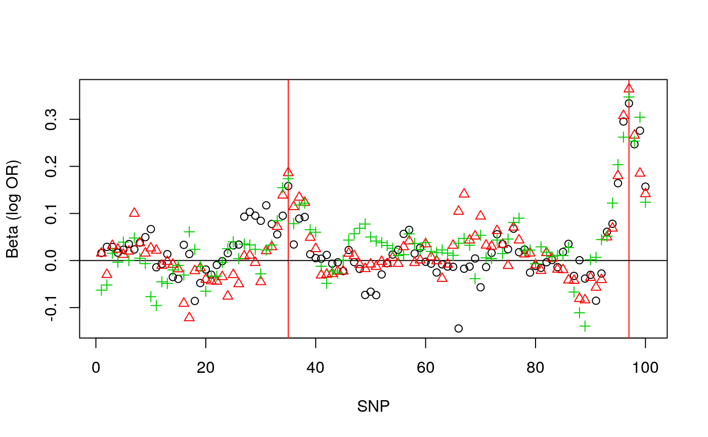
## [3,] 0.3474264 0.1738404

Again, these can be plotted, to see the variability between replicates:

plot(1:nsnps,betasim[1,],
     xlab="SNP",ylab="Beta (log OR)",
     ylim=c(min(betasim),max(betasim)))
abline(v=which(snps %in% CV),col="red"); abline(h=0)
for(i in 2:3) {
  points(1:nsnps,betasim[i,],col=i,pch=i)
}

Chris Wallace

2018-09-29

See also

Contents