DEPRECATED Coloc: relaxing the single causal variant assumption

Multiple causal variants

This describes deprecated functions - the SuSiE approach is more accurate and should be used instead

We load some simulated data.

library(coloc)

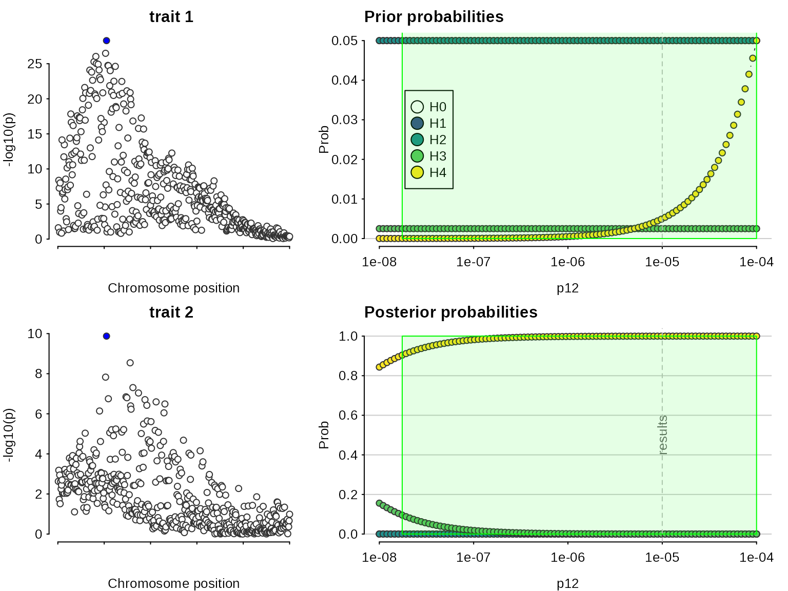
## This is coloc version 5.2.2

data(coloc_test_data)
attach(coloc_test_data) # contains D3, D4 that we will use in this vignette

First, let us do a standard coloc (single causal variant) analysis to serve as a baseline comparison. The analysis concludes there is colocalisation, because it “sees” the SNPs on the left which are strongly associated with both traits. But it misses the SNPs on the right of the top left plot which are associated with only one trait.

library(coloc)
my.res <- coloc.abf(dataset1=D3, dataset2=D4)

## PP.H0.abf PP.H1.abf PP.H2.abf PP.H3.abf PP.H4.abf 
##  8.78e-26  6.80e-07  1.53e-22  1.85e-04  1.00e+00 
## [1] "PP abf for shared variant: 100%"

class(my.res)

## [1] "coloc_abf" "list"

## print.coloc_abf
my.res

## Coloc analysis of trait 1, trait 2

## 
## SNP Priors

##    p1    p2   p12 
## 1e-04 1e-04 1e-05

## 
## Hypothesis Priors

##        H0   H1   H2       H3    H4
##  0.892505 0.05 0.05 0.002495 0.005

## 
## Posterior

##        nsnps           H0           H1           H2           H3           H4 
## 5.000000e+02 8.775708e-26 6.797736e-07 1.529399e-22 1.848705e-04 9.998144e-01

sensitivity(my.res,"H4 > 0.9")

## Results pass decision rule H4 > 0.9

Even though the sensitivity analysis itself looks good, the Manhattan plots suggest we are violating the assumption of a single causal variant per trait.
We can use =finemap.signals= to test whether there are additional signals after conditioning.

finemap.signals(D3,method="cond")

##      s105       s78 
## 11.180489  5.351394

finemap.signals(D4,method="cond")

##    s105 
## 6.42341

Note that every colocalisation conditions out every other signal except one for each trait. For that reason, trying to colocalise many signals per trait is not recommended. Instead, use pthr to set the significance (p value) required to call a signal. If you set if too low, you will capture signals that are non-significant, or too high and you will miss true signals. pthr=5e-8 would correspond to a genome-wide significance level for common variants in a European study, but we typically choose a slightly relaxed pthr=1e-6 on the basis that if there is one GW-significant signal in a region, we expect there is a greater chance for secondary signals to exist.

finemap.signals(D3,method="cond",pthr=1e-20) ## too small

##     s105 
## 11.18049

finemap.signals(D4,method="cond",pthr=0.1) ## too big

##      s105      s108      s156 
##  6.423410 -3.226812  3.741284

Now we can ask coloc to consider these as separate signals using the coloc.signals() function.

res <- coloc.signals(D3,D4,method="cond",p12=1e-6,pthr=1e-6)

## PP.H0.abf PP.H1.abf PP.H2.abf PP.H3.abf PP.H4.abf 
##  8.76e-25  6.79e-06  1.53e-21  1.85e-03  9.98e-01 
## [1] "PP abf for shared variant: 99.8%"
## PP.H0.abf PP.H1.abf PP.H2.abf PP.H3.abf PP.H4.abf 
##  1.83e-05  5.53e-04  3.19e-02  9.64e-01  3.52e-03 
## [1] "PP abf for shared variant: 0.352%"
## PP.H0.abf PP.H1.abf PP.H2.abf PP.H3.abf PP.H4.abf 
##  5.44e-04  2.33e-05  9.49e-01  4.04e-02  1.02e-02 
## [1] "PP abf for shared variant: 1.02%"

res

## Coloc analysis of trait 1, trait 2

## 
## SNP Priors

##    p1    p2   p12 
## 1e-04 1e-04 1e-06

## 
## Hypothesis Priors

##        H0   H1   H2       H3    H4
##  0.897005 0.05 0.05 0.002495 5e-04

## 
## Posterior

##    nsnps hit1 hit2           H0           H1           H2         H3
## 1:   500 s105 s105 8.674493e-25 6.719334e-06 1.511759e-21 0.01171021
## 2:   500  s78 s105 1.830995e-05 5.531424e-04 3.190992e-02 0.96399665
##             H4
## 1: 0.988283067
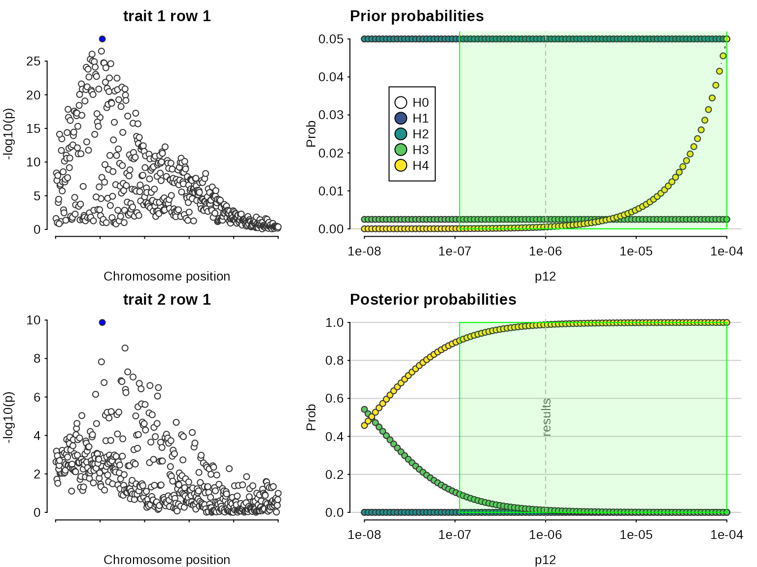
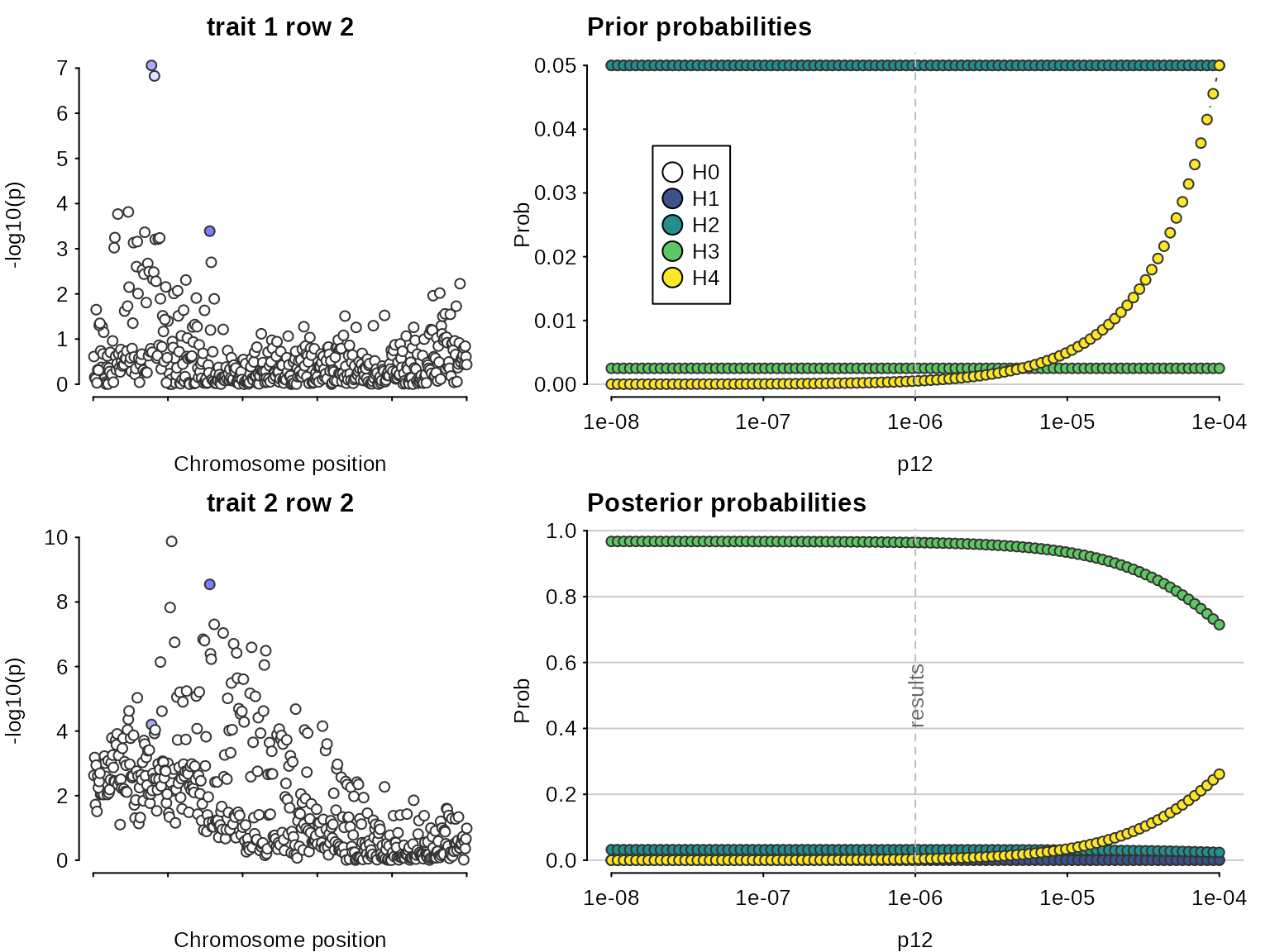
## 2: 0.003521974

Note that because we are doing multiple colocalisations, sensitivity() needs to know which to consider:

sensitivity(res,"H4 > 0.9",row=1)

## Results pass decision rule H4 > 0.9

sensitivity(res,"H4 > 0.9",row=2)

## Results fail decision rule H4 > 0.9

Chris Wallace

2023-05-12

Multiple causal variants