Test for the single-> joint linear regression calculations

Chris Wallace

2018-09-29

Joint regression back-calculation for quantitative traits

When estimated regression coefficients for two quantitative traits are not independent, because they have been estimated using the same individuals, coloc.abf() is invalid, as it assumes the joint likelihood for both traits can be partitioned into the products of likelihoods for each. Unfortunately, it is also not common to provide the joint likelihood summary statistics, and would be wasteful in terms of space. But fortunately, the summary information is usually sufficient for exact reconstruction of the joint likelihood summary statistics. This vignette demonstrates that code implementing that reconstruction works, using simulated data. A user does not need to call these functions, they are called within colocqq(). load coloc

library(coloc)
library(bindata)
library(data.table)
library(magrittr)
library(ggplot2)

The case of one SNP

here we only need to calculate var(b1,b2) where b1, b2 are the regression coefficients for traits 1 and 2 against the same SNP (which we will call X)

this is a function to simulate genotype data, calculate joint univariate regression directly, and calculate it via reconstruction from the single-trait univariate regression summary statistics.

simmer <- function() {
    maf.1 <- sample(2:10,1)/20 # snp1
    maf.2 <- sample(2:10,1)/20 # snp2
    N <- sample(c(1,2,5),1)*1000
    ## rho <- sample(c(0,0.3),1)
    rho <- 0
    mrho <- matrix(c(1, rho, rho, 1), ncol = 2)
    ## cat(maf.1,maf.2,rho,"\n")
    h1 <- rmvbin(N, margprob = c(maf.1, maf.2), bincorr = mrho)
    h2 <- rmvbin(N, margprob = c(maf.1, maf.2), bincorr = mrho)
    x <- h1 + h2
    mu1 <- sample(c(1,2,4),1)
    mu2 <- sample(c(1,2,4),1)
    y1 <- rnorm(N, x[,1] * mu1 + x[,2], sd=4)
    y2 <- rnorm(N, x[,1] * mu2 + x[,2], sd=2)
    m <- lm(cbind(y1,y2) ~ x[,1])
    m1 <- lm(y1 ~ x[,1])
    m2 <- lm(y2 ~ x[,1])

    ## summary stats
    b1 <- coef(m1)[2]
    b2 <- coef(m2)[2]
    vb1 <- vcov(m1)[2,2]
    vb2 <- vcov(m2)[2,2]
    fx <- mean(x[,1])/2
    v1 <- var(y1)
    v2 <- var(y2)
    eta=cor(y1,y2)

    res <- coloc:::qq.onesnp(b1,b2,vb1,vb2,fx,v1,v2,eta,N)*sqrt(vb1*vb2)
    names(res) <- "est.vb1b2"
    ## names(res) <- paste0("est.",names(res))
    ## target <- c(b1=b1,b2=b2,vb1=vb1,vb2=vb2,vb1b2=vcov(m)[4,2])
    target <- c(vb1b2=vcov(m)[4,2]) 
    copy(do.call("data.table",
            c(list(maf.1=maf.1,
                   maf.2=maf.2,
                   N=N,
                   eta=eta),
              as.list(target),
              as.list(res)
              )))
}

each run produces output like

simmer()  

##    maf.1 maf.2    N       eta        vb1b2    est.vb1b2
## 1:  0.45   0.3 5000 0.1455323 0.0001816654 0.0001818118

we will run it lots of times, and compare output

res <- lapply(1:100,function(i) simmer())  %>%  rbindlist()

numerically almost identical results

cor(res[,"vb1b2"],res[,"est.vb1b2"]) # 0.984

##       est.vb1b2
## vb1b2 0.9999799

ggplot(res,aes(x=vb1b2,y=est.vb1b2)) + geom_point() + geom_abline()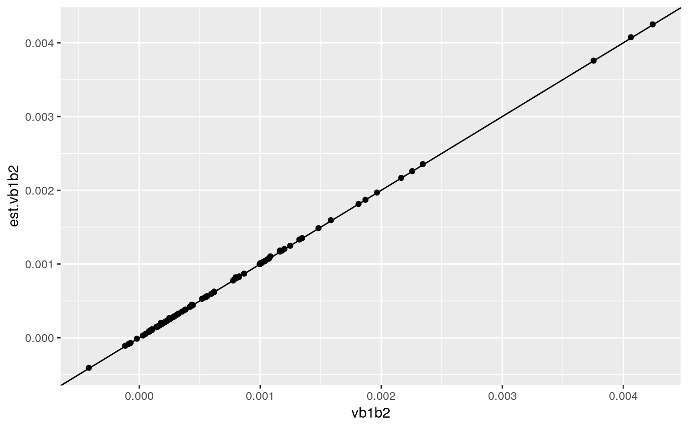 

################################################################################

now try same for joint 2 snp model from 4 univariates

simmer <- function() {
    maf.1 <- sample(2:10,1)/20 # snp1
    maf.2 <- sample(2:10,1)/20 # snp2
    N <- sample(c(1,2,5),1)*1000
    ## rho <- sample(c(0,0.3),1)
    rho <- max(maf.1,maf.2) * sample(c(0,3,5),1)/10 
    mrho <- matrix(c(1, rho, rho, 1), ncol = 2)
    ## cat(maf.1,maf.2,rho,"\n")
    h1 <- rmvbin(N, margprob = c(maf.1, maf.2), bincorr = mrho)
    h2 <- rmvbin(N, margprob = c(maf.1, maf.2), bincorr = mrho)
    x <- h1 + h2
    mu1 <- sample(c(1,2,4),1)
    mu2 <- sample(c(1,2,4),1)
    y1 <- rnorm(N, x[,1] * mu1 + x[,2], sd=4)
    y2 <- rnorm(N, x[,1] * mu2 + x[,2], sd=2)
    m <- lm(cbind(y1,y2) ~ x[,1]+x[,2])
    m11 <- lm(y1 ~ x[,1])
    m21 <- lm(y2 ~ x[,1])
    m12 <- lm(y1 ~ x[,2])
    m22 <- lm(y2 ~ x[,2])

    ## summary stats
    b1 <- coef(m11)[2]
    b2 <- coef(m21)[2]
    g1 <- coef(m12)[2]
    g2 <- coef(m22)[2]
    vb1 <- vcov(m11)[2,2]
    vb2 <- vcov(m21)[2,2]
    vg1 <- vcov(m12)[2,2]
    vg2 <- vcov(m22)[2,2]
    fx <- mean(x[,1])/2
    fz <- mean(x[,2])/2
    v1 <- var(y1)
    v2 <- var(y2)
    eta=cor(y1,y2)
    rho=cor(x[,1],x[,2])
    
    res <- coloc:::qq.twosnp(b1,b2,g1,g2,vb1,vb2,vg1,vg2,fx,fz,rho,v1,v2,eta,N)
    names(res) <- paste0("est.",names(res))
    target <- c(b1=coef(m)[2,1],
                b2=coef(m)[2,2],
                g1=coef(m)[3,1],
                g2=coef(m)[3,2],
                vb1=vcov(m)[2,2],
                vb2=vcov(m)[5,5],
                vg1=vcov(m)[3,3],
                vg2=vcov(m)[6,6],
                vb1b2=vcov(m)[2,5],
                vg1g2=vcov(m)[3,6],
                vb1g1=vcov(m)[2,3],
                vb2g2=vcov(m)[5,6],
                vb1g2=vcov(m)[2,6])
    copy(do.call("data.table",
            c(list(maf.1=maf.1,
                   maf.2=maf.2,
                   rho=rho,
                   N=N,
                   eta=eta),
              as.list(target),
              as.list(res)
              )))
}

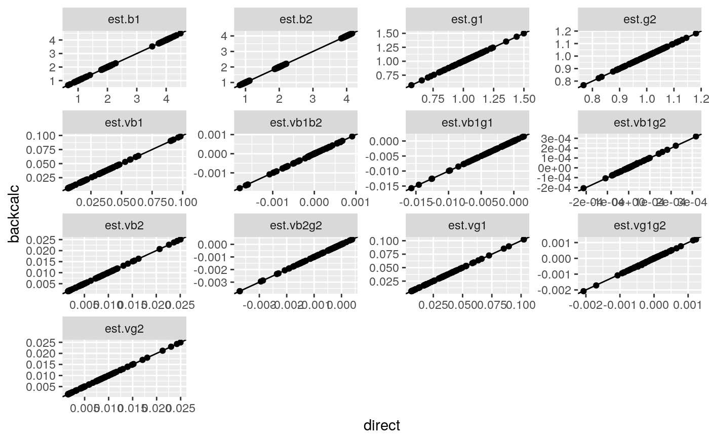
res <- lapply(1:100,function(i) simmer())  %>% rbindlist()

this time there are several quantities to calculate they still correlate very well, between directly caclulated and back-calculated

cn <- grep("est",names(res),value=TRUE)
ecn <- sub("est.","",cn)
structure(diag(cor(res[,cn,with=FALSE],res[,ecn,with=FALSE])),
          names=ecn)

##        b1        b2        g1        g2       vb1       vb2     vb1b2 
## 1.0000000 1.0000000 0.9999999 0.9999997 1.0000000 0.9999991 0.9999168 
##       vg1       vg2     vg1g2     vb1g1     vb2g2     vb1g2 
## 0.9999999 0.9999984 0.9997624 1.0000000 0.9999992 0.9998546

library(ggplot2)
tmp <- melt(res,measure.vars=list(direct=cn,backcalc=ecn))
tmp[,variable:=cn[variable]]
ggplot(tmp,aes(x=direct,y=backcalc)) + geom_point() + geom_abline() + facet_wrap(~variable,scales="free")