Coloc: proportionality testing

Chris Wallace

2021-02-19

Proportional testing

vignette: > % % %

Simulate a small dataset

library(mvtnorm)
simx <- function(nsnps,nsamples,S,maf=0.1) {
    mu <- rep(0,nsnps)
    rawvars <- rmvnorm(n=nsamples, mean=mu, sigma=S)
    pvars <- pnorm(rawvars)
    x <- qbinom(1-pvars, 2, maf)
}


sim.data <- function(nsnps=50,nsamples=200,causals=floor(nsnps/2),nsim=1) {
  cat("Generate",nsim,"small sets of data\n")
  ntotal <- nsnps * nsamples * nsim
  S <- (1 - (abs(outer(1:nsnps,1:nsnps,`-`))/nsnps))^4
  X1 <- simx(nsnps,ntotal,S)
  X2 <- simx(nsnps,ntotal,S)
  Y1 <- rnorm(ntotal,rowSums(X1[,causals,drop=FALSE]/2),2)
  Y2 <- rnorm(ntotal,rowSums(X2[,causals,drop=FALSE]/2),2)
  colnames(X1) <- colnames(X2) <- paste("s",1:nsnps,sep="")
  df1 <- cbind(Y=Y1,X1)
  df2 <- cbind(Y=Y2,X2)
  if(nsim==1) {
    return(new("simdata",
               df1=as.data.frame(df1),
               df2=as.data.frame(df2)))
  } else {
    index <- split(1:(nsamples * nsim), rep(1:nsim, nsamples))
    objects <- lapply(index, function(i) new("simdata", df1=as.data.frame(df1[i,]),
                                             df2=as.data.frame(df2[i,])))
    return(objects)
  }
}

set.seed(46411)
data <- sim.data()

## Generate 1 small sets of data

Analysis

The code below first prepares a principal component object by combining the genotypes in the two dataset, then models the most informative components (the minimum set required to capture 80% of the genetic variation) in each dataset, before finally testing whether there is colocalisation between these models.

## run a coloc with pcs
library(coloc)

## This is a new update to coloc.

pcs <- pcs.prepare(data@df1[,-1], data@df2[,-1])
pcs.1 <- pcs.model(pcs, group=1, Y=data@df1[,1], threshold=0.8)

## selecting 14 components out of 50 to capture 0.8065497 of total variance.

pcs.2 <- pcs.model(pcs, group=2, Y=data@df2[,1], threshold=0.8)

## selecting 14 components out of 50 to capture 0.8065497 of total variance.

ct.pcs <- coloc.test(pcs.1,pcs.2)
plot(ct.pcs)

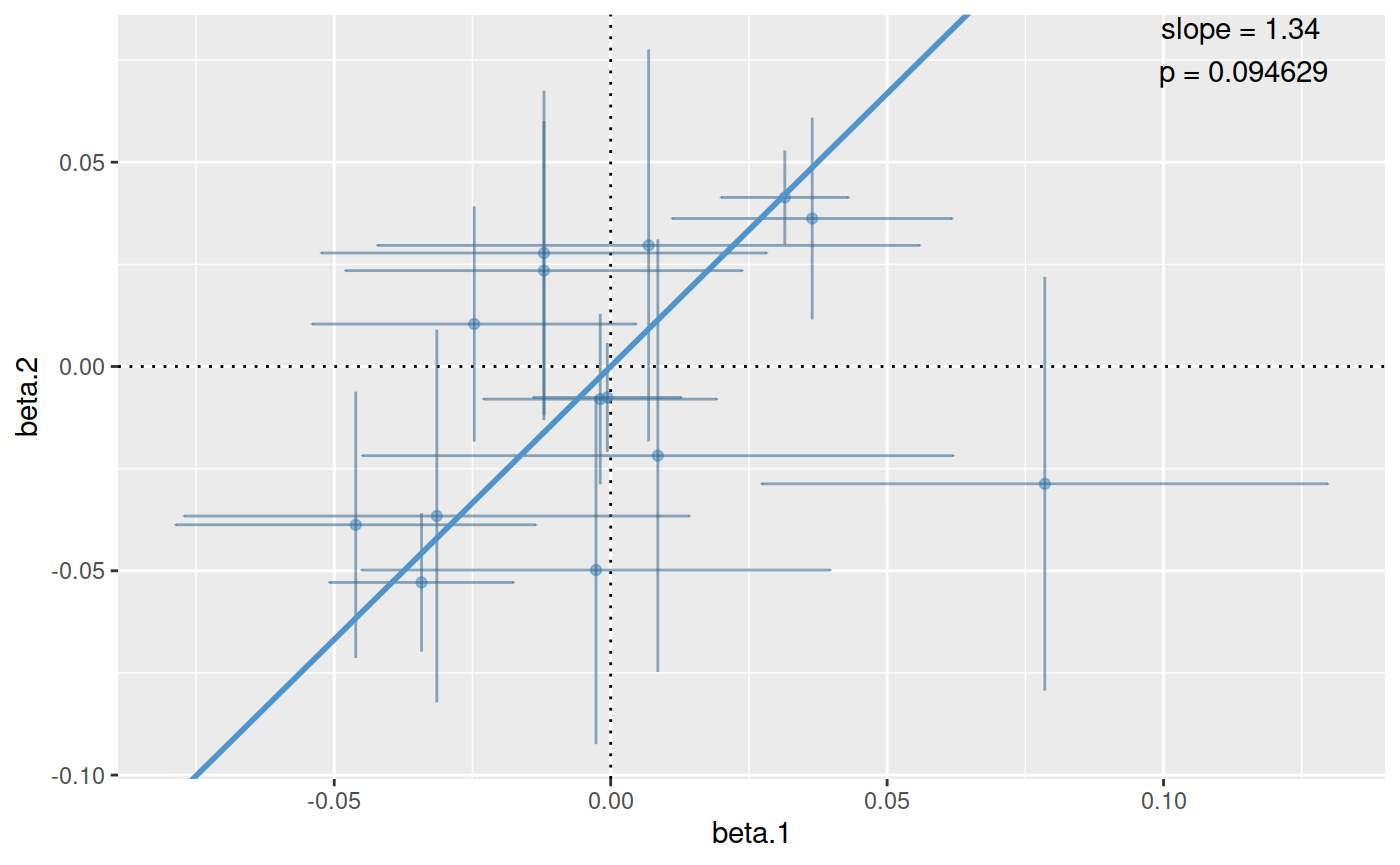
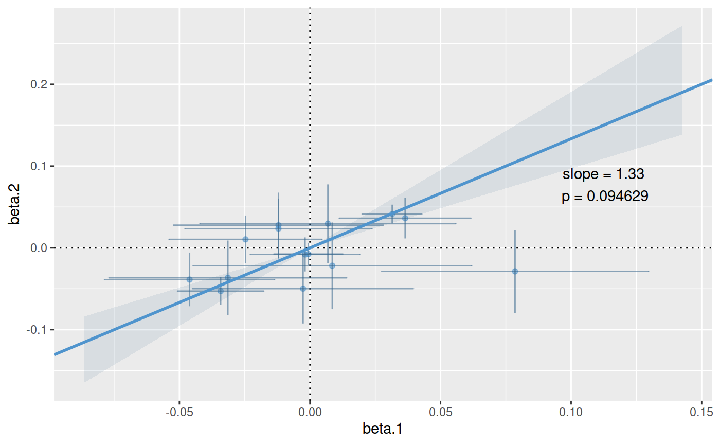
The plot shows the estimated coefficients for each principal component modeled for traits 1 and 2 on the x and y axes, with crosses showing the 95% confidence intervals. The points lie close to the line through the origin, which supports a hypothesis of colocalisation.

A little more information is stored in the ct.pcs object:

ct.pcs

##           eta.hat         chisquare                 n p.value.chisquare 
##        1.33605972       20.02337592       14.00000000        0.09462891

str(summary(ct.pcs))

##           eta.hat         chisquare                 n p.value.chisquare 
##        1.33605972       20.02337592       14.00000000        0.09462891 
##  Named num [1:4] 1.3361 20.0234 14 0.0946
##  - attr(*, "names")= chr [1:4] "eta.hat" "chisquare" "n" "p.value.chisquare"

The best estimate for the coefficient of proportionality, \(\hat{\eta}\), is 1.13, and the null hypothesis of colocalisation is not rejected with a chisquare statistic of 5.27 based on 7 degrees of freedom (\(n-1\) where the \(n\) is the number of components tested, and one degree of freedom was used in estimating \(\eta\)), giving a p value of 0.63. The summary() method returns a named vector of length 4 containing this information.

If more information is needed about \(\eta\), then this is available if the bayes argument is supplied:

ct.pcs.bayes <- coloc.test(pcs.1,pcs.2, bayes=TRUE)

## ..............

plot(ct.pcs.bayes)

ci(ct.pcs.bayes)

## $eta.mode
## [1] 1.333878
## 
## $lower
## [1] 0.9704671
## 
## $upper
## [1] 1.906443
## 
## $level.observed
## [1] 0.9469009
## 
## $interior
## [1] TRUE

Using Bayes Factors to compare specific values of \(\eta\)

It may be that specific values of \(\eta\) are of interest. For example, when comparing eQTLs in two tissues, or when comparing risk of two related diseases, the value \(\eta=1\) is of particular interest. In proportional testing, we can use Bayes Factors to compare the support for different values of \(\eta\). Eg

## compare individual values of eta
ct.pcs <- coloc.test(pcs.1,pcs.2, bayes.factor=c(-1,0,1))

## ..............

bf(ct.pcs)

##           values.against
## values.for           -1            0            1
##         -1 1.000000e+00 9.331207e-12 1.046155e-32
##         0  1.071673e+11 1.000000e+00 1.121136e-21
##         1  9.558809e+31 8.919522e+20 1.000000e+00